Jaein Land
NLP and others
20 February 2021
[Paper Notes] Complex Embeddings for Simple Link Prediction (2016) (2)
Theo Trouillon, Johannes Welbl, Sebastian Riedel, Eric Gaussier, Guillaume Bouchard
Keywords: NLP, Link Prediction, Embedding Model, Complex Embedding
Statement: I recently started posting paper reviews in my blog for my research on NLP. However, I am not yet a professional researcher as well as English is not my native language so that my posts might have some incorrect descriptions. I hope whoever reading my post understand my situation and I will be very grateful if you correct any wrong information. <3 The comment section will be added to my blog very soon!!
This post is about the theoretical stuff involved in the paper. If you want to get the general idea of this paper, please read this post.
Intuitions of the modeling
So what I wanted to understand is: (1) why the complex embeddings are needed and (2) why eigenvalue decomposition rather than SVD. The author applied complex embeddings on a simplified link prediction task with a single relation type to introduce the intuition of using it.
Let’s learn some definitions first:
- $\varepsilon$ is a set of entities with |${\varepsilon}$|=$n$.
- A relation between two entities is binary value $Y_{so}\in \{-1, 1\}$, where $s, o\in{\varepsilon}$. — (1)
- $s, o$ represents subject and object respectively.
The goal is to find a latent matrix $X\in{\mathbb{R}}^{n\times n}$, which is a score matrix between entities. $Y$ is the partially observed sign matrix. There are many existing matrix factorization approaches, such as SVD, to approximate $X$. However, we have to notice that the same entity can appear as both subject and object. Naturally, joint embeddings of the entities are learnt in most of link prediction research. For example, Eigenvalue decomposition is often used to approximate real symmetric matrices such as similarity matrices:
But how to make it possible to also be antisymmetric? It is not possible in the real space! This could be why the complex embeddings are used in this research. With complex numbers, the dot product is defined as:
where $u$ and $v$ are complex vectores. Specifically, $u=Re(u)+iIm(u)$ with $Re(u)\in{\mathbb{R}^K}$ and $Im(u)\in{\mathbb{R}^K}$. Also, to avoid the computational issues eigendecomposition, the space of normal matrices is considered. A matrix $X$ is normal if and only if it is unitarily diagonalizable. So that let’s re-define the matrix $X$ as:
where $W$ is the diagonal matrix of eigenvalues, $E$ is a unitary matrix of eigenvectors with $\bar{E}$ representing its complex conjugate($W, E\in{\mathbb{C}^{n\times n}}$). Then, to satisfy equation 1, only the real part of the decompostion is used.
The eigenvalue decomposition brings us two advantages:
- The eigenvalues are not necessarily positive or real;
- The rows of $E$ can be used as vectorial representations of the entities corresponding to rows and columns of the relation matrix $X$. For an entity, its subject embedding vector is the complex conjugate of its object embedding vector.
Learnable Model
In a link prediction task, only partial information is given and we want to find the rest relations to complete the relation matrix. What we want to make learnable is the relation score between two entities. Assuming the binary relations have low sign-rank, individual relation scores $X_{so}$ can be predicted through:
In brief conclusion, the learnable relations can be efficiently approximated by a simple low-rank factorization using complex numbers to represent the latent factors.
Applying to Binary Multi-Relational Data
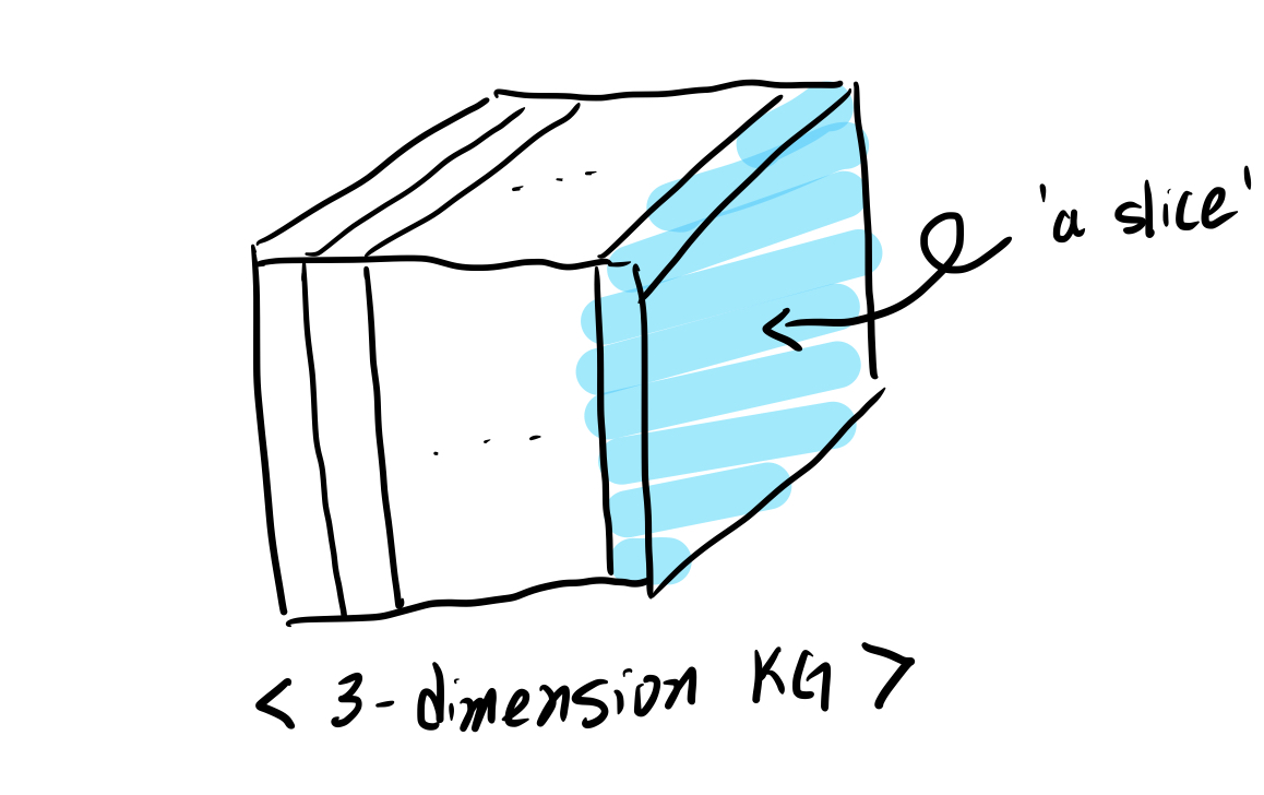
In above contents, we were focusing on a single relationship, which you can imagine as one ‘slice’ of the 3D KG. Since we learnt the intuition of this paper with a single ‘slice’, now let’s see the application to the entire 3D KG, the multi-relational data.

The probability that the fact $r(s,0) is true is:
where $\phi$ is a scoring function based on a factorization of the observed relations, $\Theta$ denotes the parameters of the corresponding model. The goal is to determine entries ${\textbf{Y}}$ being true or farse for a set of targeted unobserved triples. $\sigma$ is a scoring function used to predict the entries of the tensor $\textbf{X}$.
Briefly, the final model scoring function is a improved version of DistMult by adding complex values. With the score function, it is easy to check if one is symmetric or antisymettir. For example, if there exists $<e_o,e_s>=<\bar{e_s,e_o}>$, it indicates that $Re(<e_o,e_s>)$ is symmetric, while $Im(e_o,e_s)$ is antisymmetric.
In conclusion, this approach can accurately describe both symmetric and antisymmetric while still using joint representations whether they appear as subject of object of relations. The author demostrated its effectiveness by using FB15K and WN18 datasets. And the experimental results show that ComplEx outperforms standard link prediction benchmarks.
If you are interested in detailed theories of this paper, I suggest you to read the original paper!